Acknowledgements
References for this Material:
- Treedata book by Guangchuang Yu (Yu 2022) https://yulab-smu.top/treedata-book/
- https://bioconnector.github.io/workshops/r-ggtree.html
Learning objectivesx
At the end of this lesson you will:
- Understand information content of phylogenetically structured data
- Understand particular R tree formats in ape, phylobase, and ouch
- Be able to hand-make trees
- Be able to import trees from nexus, newick, and other major formats in use today
- Be able to convert trees from one format to another
- Be able to perform basic tree manipulations
apeggtreetidytreetreeioTDbookggplot2ouch
Overview
ggtree is a powerful phylogenetic tree plotting package, that is used alongside treeio and tidytree packages to import/export and to manipulate phylogenetic trees, respectively. These packages allow you to subset or combine trees with data, annotate, and plot in so many different ways using the grammar of graphics.
Because itʻs written in the style of ggplot2 and the tidyverse, there are a lot of functions to remember, and now there are also multiple object types. The key to working effectively with ggtree is to be aware of what type of object you are working with, whether it is a dataframe, a tibble, a phylo tree, a treedata tibble, or ggtree object. It is easy to convert between these at will if you know what you are dealing with.
phylo -> treedata
Functions like read.tree amd read.nexus, etc. will read in objects of class phylo (they are actually referencing the ape function).
To show this, letʻs first generate a random tree using ape::rtree()
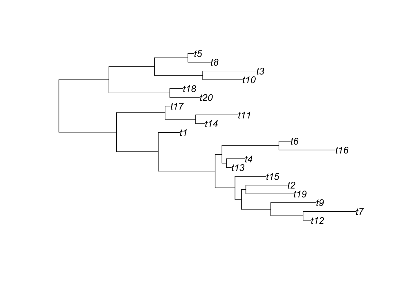
Note: ggtree can also accept phylo objects as arguments:
ggtree(tree) # ggtree plotting function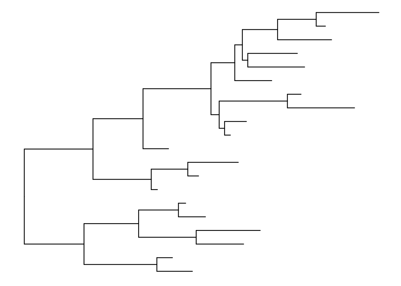
To save as newick and nexus formats, treeio has the following:
treeio::write.nexus(tree, file="tree.nex")
treeio::write.tree(tree, file="tree.tree")
list.files()
[1] "_index.qmd" "anolis.SSD.raw.csv" "bigtree.nex"
[4] "ggtree_functions.R" "ggtree.R" "inclass.R"
[7] "index 2.html" "index 3.html" "index_files"
[10] "index_files 2" "index_files 3" "index.qmd"
[13] "index.rmarkdown" "tree.nex" "tree.tree" Take a look at these files. They should be in nexus and newick formats, respectively.
tree_nex <- treeio::read.nexus(file="tree.nex")
tree_new <- treeio::read.newick(file="tree.tree")
class(tree_nex)
[1] "phylo"class(tree_new)[1] "phylo"If you have trees from iqtree, BEAST etc., you should use the specialized read functions because they will capture the metadata embedded in the treeformat including support values.
Coverting between data types
The main functions for coersion are:
as.phylo (tree) # to phylo
Phylogenetic tree with 20 tips and 19 internal nodes.

Tip labels:
  t12, t7, t9, t19, t2, t15, ...

Rooted; includes branch length(s).as.treedata(tree) # to treedata'treedata' S4 object'.
...@ phylo:
Phylogenetic tree with 20 tips and 19 internal nodes.
Tip labels:
t12, t7, t9, t19, t2, t15, ...
Rooted; includes branch length(s).treedata <- as.treedata(tree)
as_tibble(treedata) # to tibble# A tbl_tree abstraction: 39 × 4
# which can be converted to treedata or phylo
# via as.treedata or as.phylo
parent node branch.length label
<int> <int> <dbl> <chr>
1 28 1 0.126 t12
2 28 2 0.858 t7
3 27 3 0.739 t9
4 29 4 0.777 t19
5 29 5 0.678 t2
6 25 6 0.505 t15
7 31 7 0.0796 t13
8 31 8 0.298 t4
9 32 9 0.918 t16
10 32 10 0.186 t6
# ℹ 29 more rowsSimulate phenotypic data
Add tiplabels
ggtree(tree) + geom_tiplab()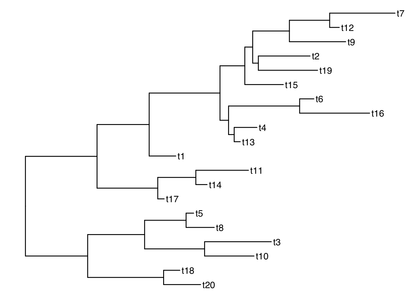
Get the tip labels
There is a function get_taxa_name() which is very handy, but NOTE: its argument is a ggtree object, not a treedata object.
p <- ggtree(tree) + geom_tiplab()
get_taxa_name(p)
[1] "t7" "t12" "t9" "t2" "t19" "t15" "t6" "t16" "t4" "t13" "t1" "t11"
[13] "t14" "t17" "t5" "t8" "t3" "t10" "t18" "t20"taxa <- get_taxa_name(p)Simulate a data matrix:
n <- length(taxa)
size <- rnorm(n, mean=20, sd=5)
habitat <- sample(c("desert", "grassland", "forest", "intertidal"), size=n, replace=T)
dat <- data.frame( "label"= taxa, size, habitat)
dat
label size habitat
1 t7 27.31979 grassland
2 t12 17.49969 intertidal
3 t9 25.84548 intertidal
4 t2 18.95584 grassland
5 t19 12.70653 grassland
6 t15 26.57089 intertidal
7 t6 24.52070 grassland
8 t16 16.90068 intertidal
9 t4 14.76381 desert
10 t13 18.01091 forest
11 t1 13.15498 desert
12 t11 15.87049 forest
13 t14 22.16129 grassland
14 t17 29.33694 intertidal
15 t5 17.23589 desert
16 t8 19.64449 grassland
17 t3 18.13256 intertidal
18 t10 16.09163 grassland
19 t18 15.60060 forest
20 t20 28.37008 desertSee our ggtree as a treedata object:
as.treedata(p) %>% as_tibble %>% as.data.frame parent node branch.length label
1 28 1 0.12604366 t12
2 28 2 0.85758925 t7
3 27 3 0.73859272 t9
4 29 4 0.77725659 t19
5 29 5 0.67810274 t2
6 25 6 0.50529245 t15
7 31 7 0.07960503 t13
8 31 8 0.29836242 t4
9 32 9 0.91839353 t16
10 32 10 0.18644255 t6
11 23 11 0.34923135 t1
12 34 12 0.14742050 t14
13 34 13 0.69041944 t11
14 33 14 0.08418970 t17
15 36 15 0.48554606 t20
16 36 16 0.21289598 t18
17 38 17 0.64849655 t10
18 38 18 0.87546294 t3
19 39 19 0.36946746 t8
20 39 20 0.09897118 t5
21 21 21 NA <NA>
22 21 22 0.93988578 <NA>
23 22 23 0.68403471 <NA>
24 23 24 0.92950240 <NA>
25 24 25 0.32552795 <NA>
26 25 26 0.10354338 <NA>
27 26 27 0.48173284 <NA>
28 27 28 0.52835976 <NA>
29 26 29 0.07430939 <NA>
30 24 30 0.11220974 <NA>
31 30 31 0.07390028 <NA>
32 30 32 0.93289393 <NA>
33 22 33 0.79672138 <NA>
34 33 34 0.49979389 <NA>
35 21 35 0.81705673 <NA>
36 35 36 0.99640114 <NA>
37 35 37 0.74696515 <NA>
38 37 38 0.78720907 <NA>
39 37 39 0.54443343 <NA> # ggtree -> treedata -> tibble -> dataframeMerge tree with data
Now that we have a matching key in both the tree and data objects, we can join the tree with the dataframe by those matching labels using ggtreeʻs full_join:
ttree <- full_join(tree, dat, by = "label")
ttree
'treedata' S4 object'.
...@ phylo:
Phylogenetic tree with 20 tips and 19 internal nodes.
Tip labels:
t12, t7, t9, t19, t2, t15, ...
Rooted; includes branch length(s).
with the following features available:
'', 'size', 'habitat'.
# The associated data tibble abstraction: 39 × 5
# The 'node', 'label' and 'isTip' are from the phylo tree.
node label isTip size habitat
<int> <chr> <lgl> <dbl> <chr>
1 1 t12 TRUE 17.5 intertidal
2 2 t7 TRUE 27.3 grassland
3 3 t9 TRUE 25.8 intertidal
4 4 t19 TRUE 12.7 grassland
5 5 t2 TRUE 19.0 grassland
6 6 t15 TRUE 26.6 intertidal
7 7 t13 TRUE 18.0 forest
8 8 t4 TRUE 14.8 desert
9 9 t16 TRUE 16.9 intertidal
10 10 t6 TRUE 24.5 grassland
# ℹ 29 more rows parent node branch.length label size habitat
1 28 1 0.12604366 t12 17.49969 intertidal
2 28 2 0.85758925 t7 27.31979 grassland
3 27 3 0.73859272 t9 25.84548 intertidal
4 29 4 0.77725659 t19 12.70653 grassland
5 29 5 0.67810274 t2 18.95584 grassland
6 25 6 0.50529245 t15 26.57089 intertidal
7 31 7 0.07960503 t13 18.01091 forest
8 31 8 0.29836242 t4 14.76381 desert
9 32 9 0.91839353 t16 16.90068 intertidal
10 32 10 0.18644255 t6 24.52070 grassland
11 23 11 0.34923135 t1 13.15498 desert
12 34 12 0.14742050 t14 22.16129 grassland
13 34 13 0.69041944 t11 15.87049 forest
14 33 14 0.08418970 t17 29.33694 intertidal
15 36 15 0.48554606 t20 28.37008 desert
16 36 16 0.21289598 t18 15.60060 forest
17 38 17 0.64849655 t10 16.09163 grassland
18 38 18 0.87546294 t3 18.13256 intertidal
19 39 19 0.36946746 t8 19.64449 grassland
20 39 20 0.09897118 t5 17.23589 desert
21 21 21 NA <NA> NA <NA>
22 21 22 0.93988578 <NA> NA <NA>
23 22 23 0.68403471 <NA> NA <NA>
24 23 24 0.92950240 <NA> NA <NA>
25 24 25 0.32552795 <NA> NA <NA>
26 25 26 0.10354338 <NA> NA <NA>
27 26 27 0.48173284 <NA> NA <NA>
28 27 28 0.52835976 <NA> NA <NA>
29 26 29 0.07430939 <NA> NA <NA>
30 24 30 0.11220974 <NA> NA <NA>
31 30 31 0.07390028 <NA> NA <NA>
32 30 32 0.93289393 <NA> NA <NA>
33 22 33 0.79672138 <NA> NA <NA>
34 33 34 0.49979389 <NA> NA <NA>
35 21 35 0.81705673 <NA> NA <NA>
36 35 36 0.99640114 <NA> NA <NA>
37 35 37 0.74696515 <NA> NA <NA>
38 37 38 0.78720907 <NA> NA <NA>
39 37 39 0.54443343 <NA> NA <NA>And thatʻs what our treedata object looks like flattened out!
Subsetting the tree
Functions: drop.tip() and keep.tip()
Suppose we want to drop all of the even tips:
todrop <- paste("t", 1:10*2, sep="")
todrop
[1] "t2" "t4" "t6" "t8" "t10" "t12" "t14" "t16" "t18" "t20"smalltree <- drop.tip(ttree, todrop)
smalltree'treedata' S4 object'.
...@ phylo:
Phylogenetic tree with 10 tips and 9 internal nodes.
Tip labels:
t7, t9, t19, t15, t13, t1, ...
Rooted; includes branch length(s).
with the following features available:
'', 'size', 'habitat'.
# The associated data tibble abstraction: 19 × 5
# The 'node', 'label' and 'isTip' are from the phylo tree.
node label isTip size habitat
<int> <chr> <lgl> <dbl> <chr>
1 1 t7 TRUE 27.3 grassland
2 2 t9 TRUE 25.8 intertidal
3 3 t19 TRUE 12.7 grassland
4 4 t15 TRUE 26.6 intertidal
5 5 t13 TRUE 18.0 forest
6 6 t1 TRUE 13.2 desert
7 7 t11 TRUE 15.9 forest
8 8 t17 TRUE 29.3 intertidal
9 9 t3 TRUE 18.1 intertidal
10 10 t5 TRUE 17.2 desert
# ℹ 9 more rowsggtree(smalltree) + geom_tiplab()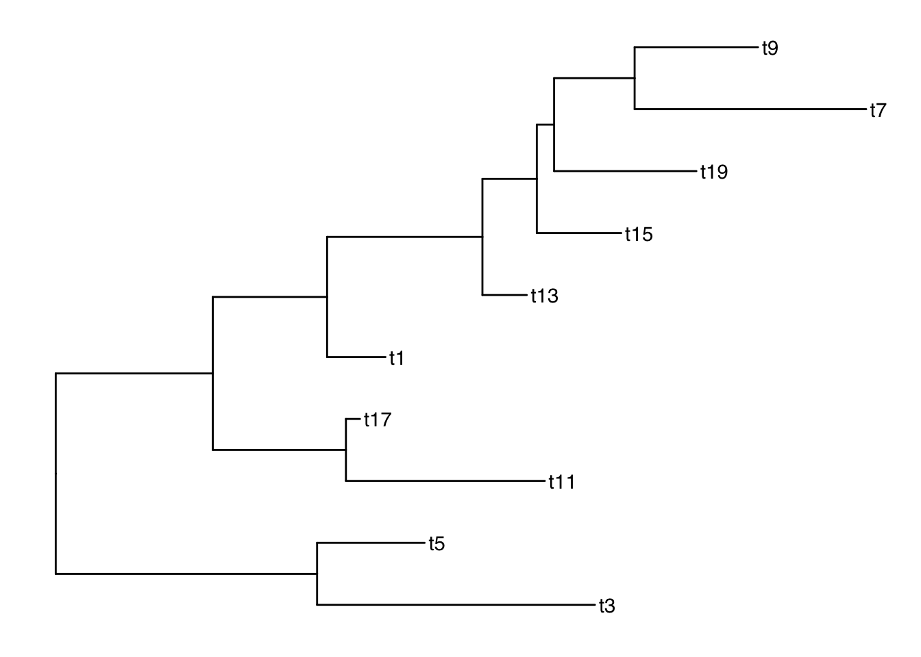
drop.tip keeps all of the metadata! keep.tip is imported from ape so it has to be converted to phylo and then the data joined again after.
Plotting with node labels
The geometries geom_text() and geom_node() are helpful for labelling all of the nodes. The function geom_tiplab() labels only the tips.
Add node labels so you know what the internal node numbers are:
ggtree(smalltree) +
    geom_tiplab() +
    geom_text(aes(label=node), hjust=-.3)    # node numbers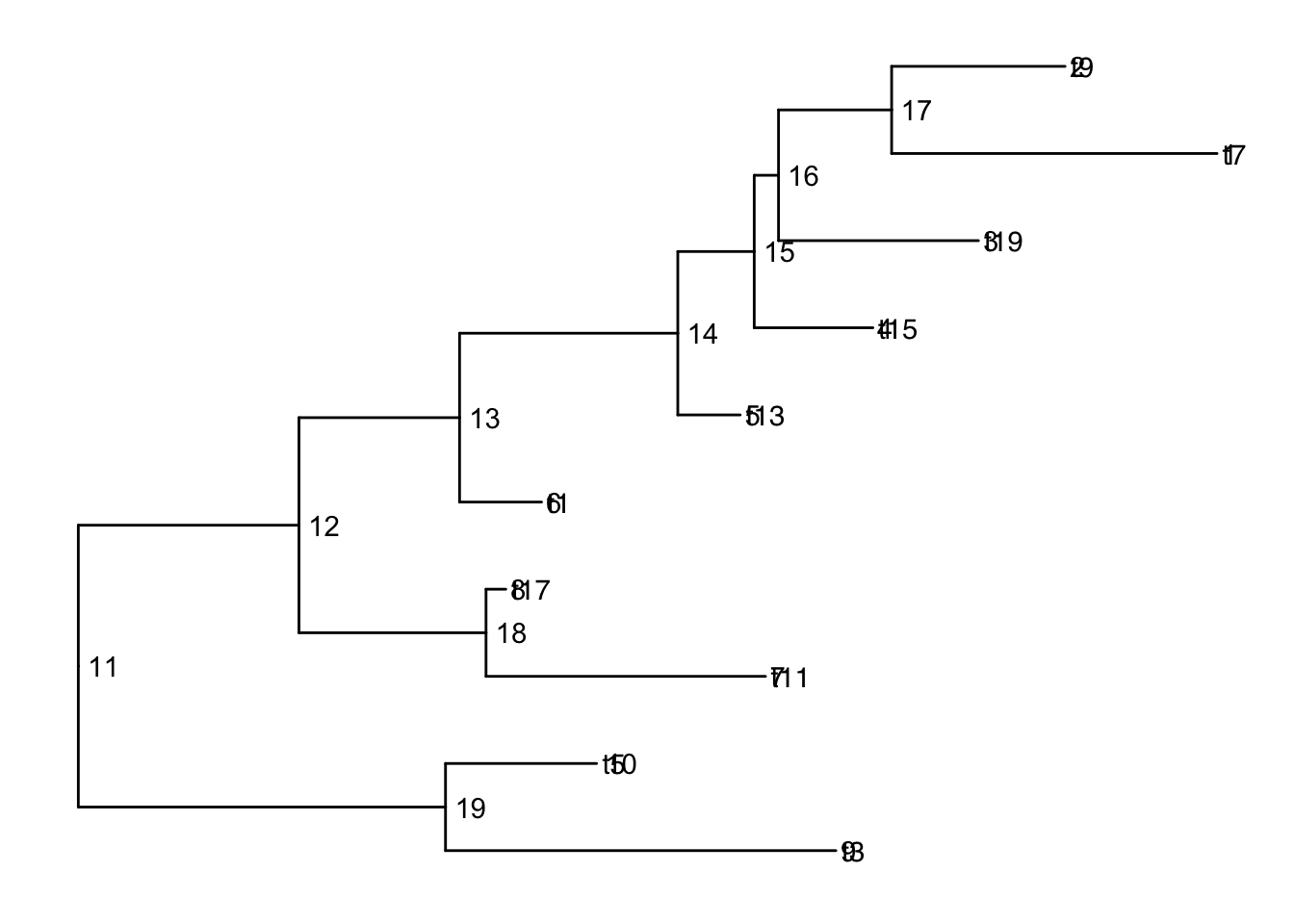
Note: The tiplabels and the node labels crashed!
There are also 2 versions: geom_text2() and geom_node2() that allow subsetting the nodes, when you want the geometry to apply to only some of the nodes.
ggtree(smalltree) +
    geom_tiplab() +
    geom_text2(aes(label=node, subset=!isTip), hjust=-.3)    # node numbers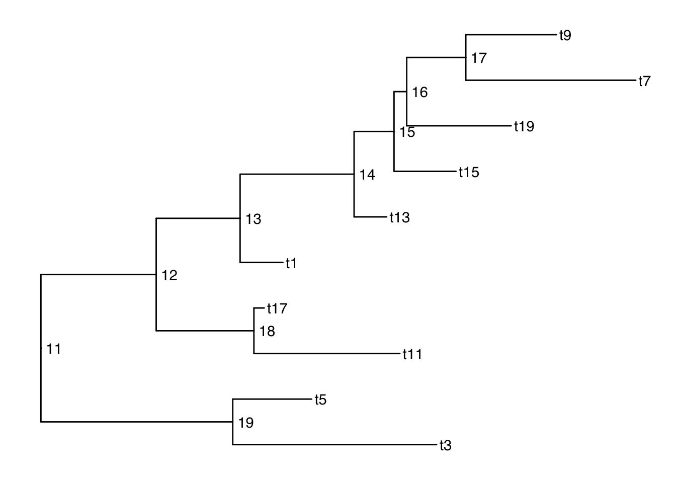
isTip is a column of the ggtree object, so it is inherited when we provide the ggtree object.
Plotting with alternative tip labels
The dataframe portion of the treedata object can hold any number of columns of metadata. Perhaps you have some real names in a different column (like a display name), it is easy to swap out the tip labels. Here letʻs just use the habitat column
ggtree(smalltree) +
    geom_tiplab(aes(label=habitat)) +
    geom_text2(aes(label=node, subset=!isTip), hjust=-.3)    # node numbers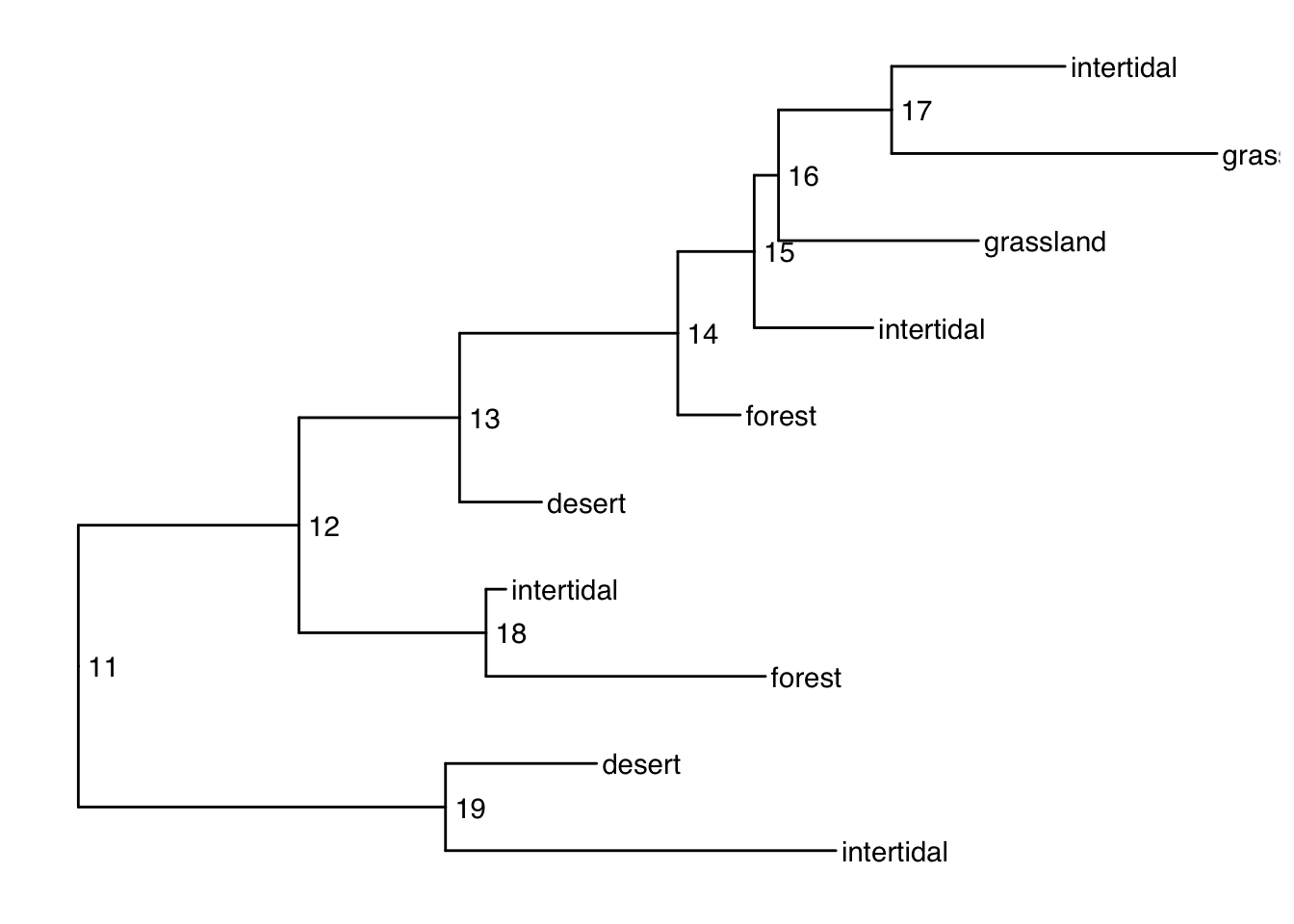
When your tip labels get cut off
Add an x scale (usually time):
ggtree(smalltree) +
    geom_tiplab(aes(label=habitat)) +
    geom_text2(aes(label=node, subset=!isTip), hjust=-.3) +   # node numbers
    theme_tree2()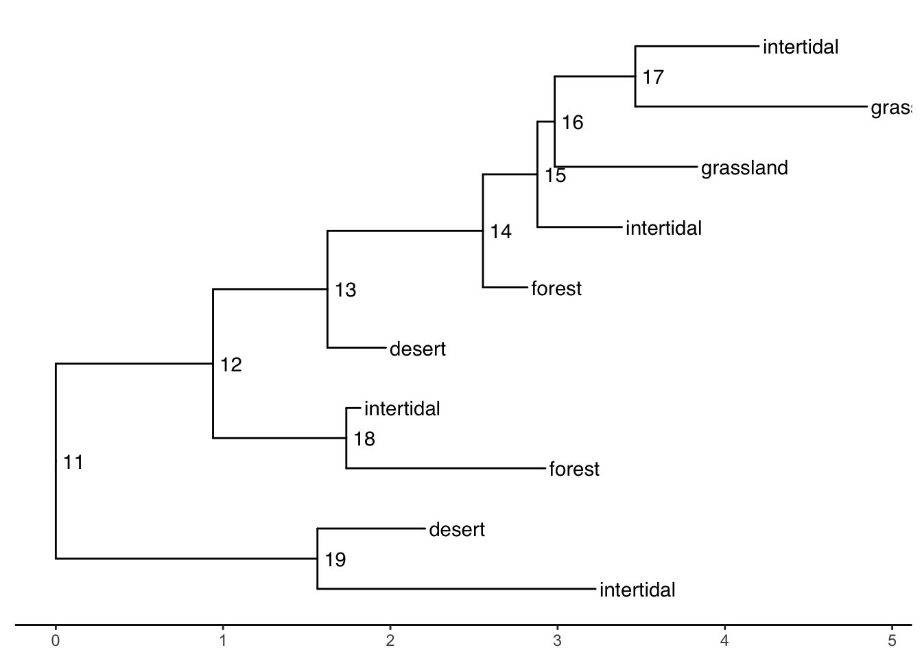
You can increase the size of the plot area to accommodate the longer labels:
ggtree(smalltree) +
    geom_tiplab(aes(label=habitat)) +
    geom_text2(aes(label=node, subset=!isTip), hjust=-.3) +   # node numbers
    theme_tree2() +
    xlim(0,5)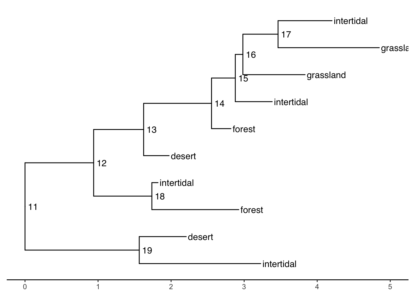
Tree layouts
require(cowplot)

plot_grid(
  ggtree(ttree),
  ggtree(ttree, branch.length='none'),
  ggtree(ttree, layout="dendrogram"),
  ggtree(ttree, layout="roundrect"),
  ggtree(ttree, layout="ellipse"),
  ggtree(ttree, layout="ellipse", branch.length="none"),
  ggtree(ttree, layout="circular"),
  ggtree(ttree, branch.length='none', layout='circular'),
  ggtree(ttree, layout="fan", open.angle=120),
  ggtree(ttree, layout="inward_circular")
)
Plotting data on the tree
geom_facet() and facet_plot() are general methods to link graphical layers to a tree.
These functions require an input dataframe with the first column containing the taxon labels (the key which matches to the tip labels of the phylogeny).
Internally these functions reorder the input data based on the tree structure so that you donʻt have to worry about the order of the rows.
Multiple layers can be added to the same dataset. Also different datasets can be added to the same figure.
A table of the geom layers that work with geom_facet is provided here.
Example: plot smalltree with size in a barplot
First make a tibble to attach to the tree. As of this writing, geom_facet will not accept a treedata object. It wants a dataframe or tibble of only the tips. But this is easy to make from the treedata. We just have to filter out the non-tip rows, then rearrange the columns to put the labels first:
We can then add the barplot as a panel next to the tree plot using geom_facet:
ggtree(smalltree) +
    geom_tiplab() +
    theme_tree2()  +
    geom_facet(panel = "Size",
               data=smdat,
               geom = geom_col,
               mapping=aes(x = smdat$size),
               orientation = 'y',
               width = .6,
fill="blue") 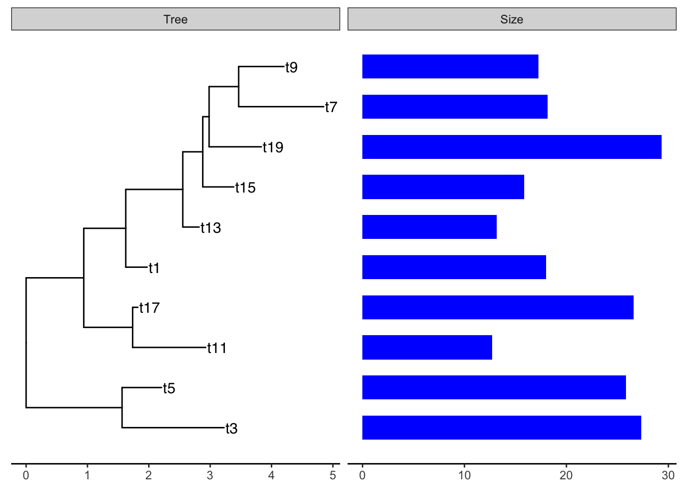
The arguments for geom_facet() are:
-
panel: The name of the panel, displayed on top -
data: atibbleordataframecontaining the metadata to plot. Must have as the first column the tip labels that are found in the phylogenetic tree. -
geom: a geom layer specifying the style of plot -
mapping: the aesthetic mapping. I should not have to supply thesmdat$here but it wonʻt work otherwise. - any additional parameters for the plot
A tree-panel and annotation example from the Tree Data Book:
This example plots a phylogeny alongside SNP (single nucleotide polymorphism) data and a barplot of some simulated data (Yu 2022).
The %+>% operator for ggtree objects
The %+>% operator is used to add data (dataframe, tibble) to a ggtree object:
my_ggtree <- my_ggtree %<+% new_dataThe result is a combined object that can be used for plotting, but it does not modify the original treedata object (which is a different object from the ggtree object). The full_join() function can be used to combine a tree with data to produce a new treedata object.
Example of the %+>% operator to add data to a ggtree object.
The package TDbook is the data accompanyment to (Yu 2022)ʻs Tree Data book. It is available on CRAN so you can install it with the usual install.packages("TDbook") function call.
p <- ggtree(tree_boots) %<+% df_tip_data + xlim(-.1, 4)
p2 <- p + geom_tiplab(offset = .6, hjust = .5) +
    geom_tippoint(aes(shape = trophic_habit, color = trophic_habit,
                size = mass_in_kg)) +
    theme(legend.position = "right") +
    scale_size_continuous(range = c(3, 10))

p2 %<+% df_inode_data +
    geom_label(aes(label = vernacularName.y, fill = posterior)) +
    scale_fill_gradientn(colors = RColorBrewer::brewer.pal(3, "YlGnBu"))
Warning: Removed 7 rows containing missing values or values outside the scale range
(`geom_label()`).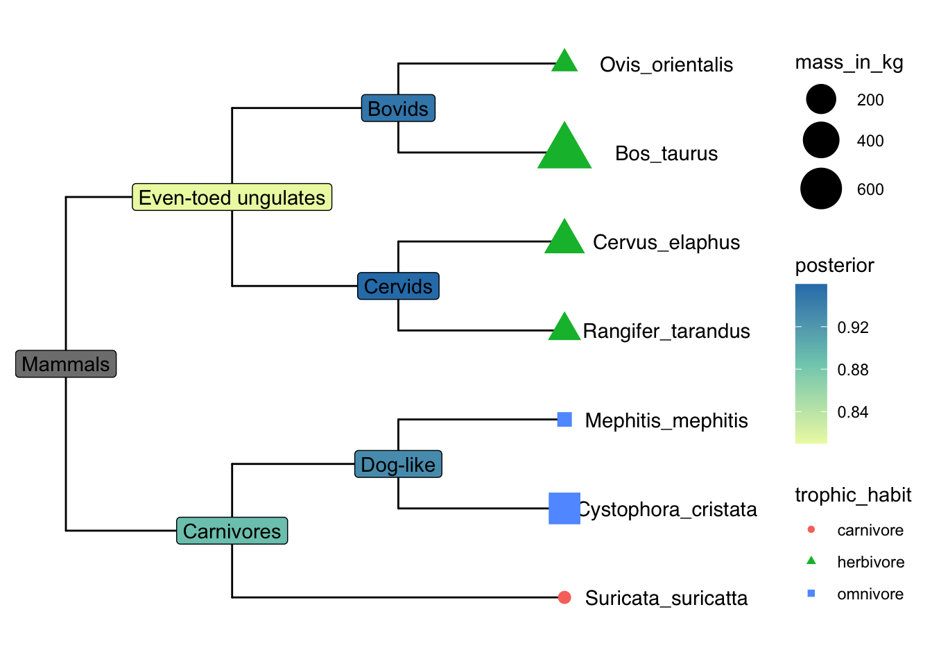
Explore df_info
df_info A dataframe containing sampling info for the tips of the tree. 386 rows and 6 variables, with the first column being taxa labels (id).
df_alleles The allele table with original raw data to be processed to SNP data. It is a table of nucleotides with 386 rows x 385 variables. The first row contains tips labels. Column names are non-sense. The rownames (exept for the first one) contains the snp position along the genome.
## load `tree_nwk`, `df_info`, `df_alleles`, and `df_bar_data` from 'TDbook'
tree <- tree_nwk
snps <- df_alleles
snps_strainCols <- snps[1,]
snps<-snps[-1,] # drop strain names
colnames(snps) <- snps_strainCols

gapChar <- "?"
snp <- t(snps)  # not rectangular!
lsnp <- apply(snp, 1, function(x) {
        x != snp[1,] & x != gapChar & snp[1,] != gapChar
    })  # different from row 1, not missing
lsnp <- as.data.frame(lsnp)
lsnp$pos <- as.numeric(rownames(lsnp))  # position from rownames
lsnp <- tidyr::gather(lsnp, name, value, -pos)
snp_data <- lsnp[lsnp$value, c("name", "pos")] # only TRUEs
snp_data A dataframe containing SNP position data. 6482 x 2. The first column contains taxa labels coresponding to the tips of the tree (name). There are multiple rows per taxon, the second colum is the position pos of the snp in the genome. This is used as the x-variable in the plot.
In the dataframe snp_data the rows are ordered by position along the sequence (the x-dimension of this data), but the first column is the strain (taxon) name which matches the tips in the phylogenetic tree.
## visualize the tree
p <- ggtree(tree)

## attach the sampling information data set
## and add symbols colored by location
p <- p %<+% df_info + geom_tippoint(aes(color=location))
p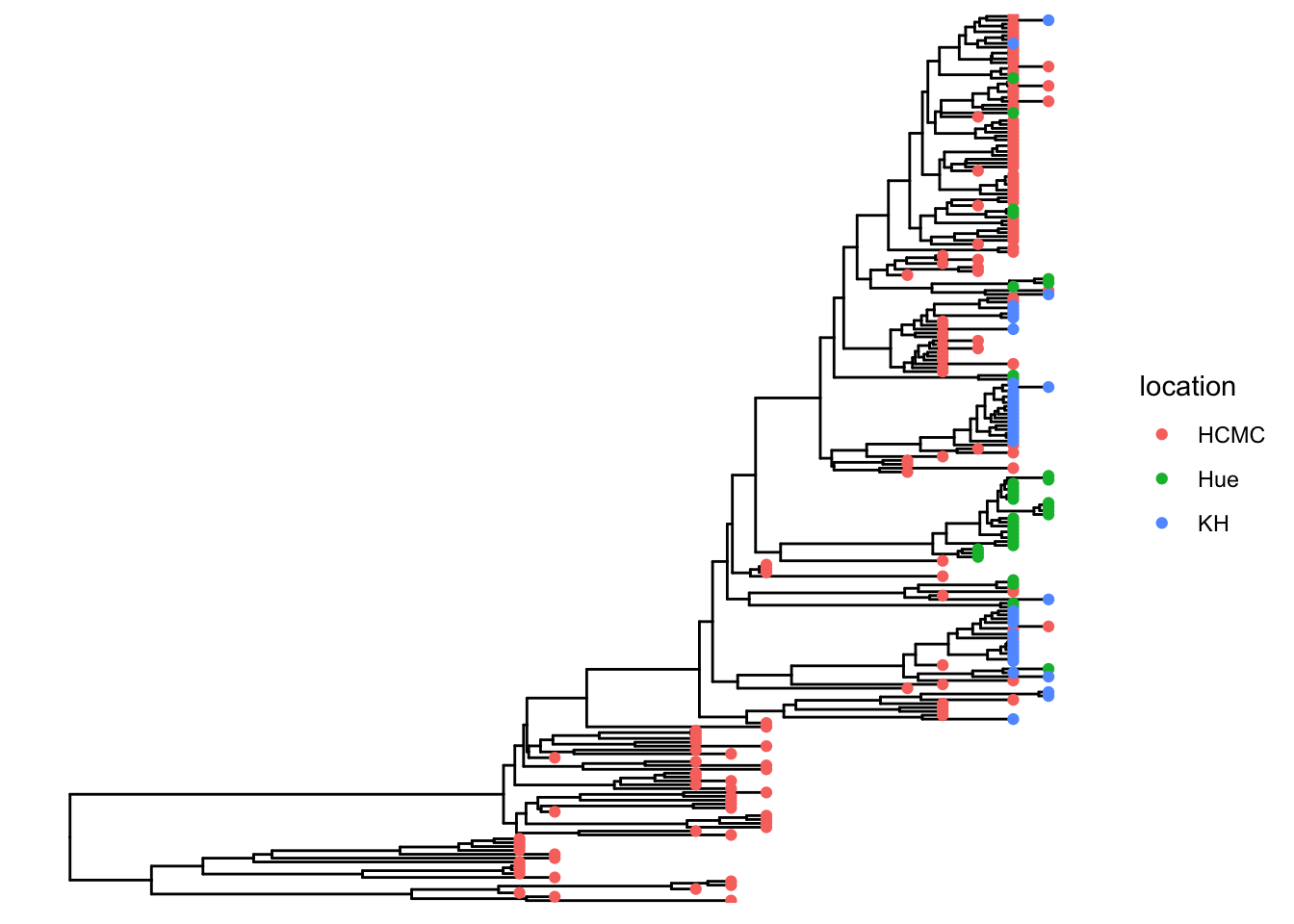
Add SNP and Trait plots aligned to the tree
Use geom_facet with reference to the respective dataframes/tibbles to add plots alignted to the tree. For the SNP plot, we will use geom_point which allows x-y plotting, with x-coordinate determined by pos and the y-coordinate aligned with the taxon. The symbol is the vertical line |.
## visualize SNP and Trait data using dot and bar charts,
## and align them based on tree structure
p1 <- p + geom_facet(panel = "SNP", data = snp_data, geom = geom_point,
               mapping=aes(x = pos, color = location), shape = '|')
p1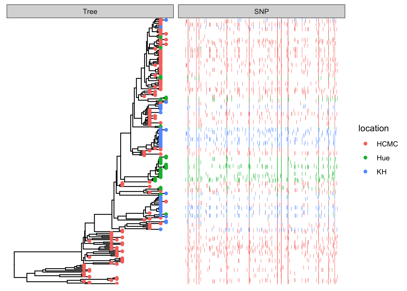
df_bar_data is some simulated data with an id column specifying the taxon names, and a dummy_bar_value containing some data.
p1 + geom_facet(panel = "Trait", data = df_bar_data, geom = geom_col,
                aes(x = dummy_bar_value, color = location,
                fill = location), orientation = 'y', width = .6) +
    theme_tree2(legend.position=c(.05, .85))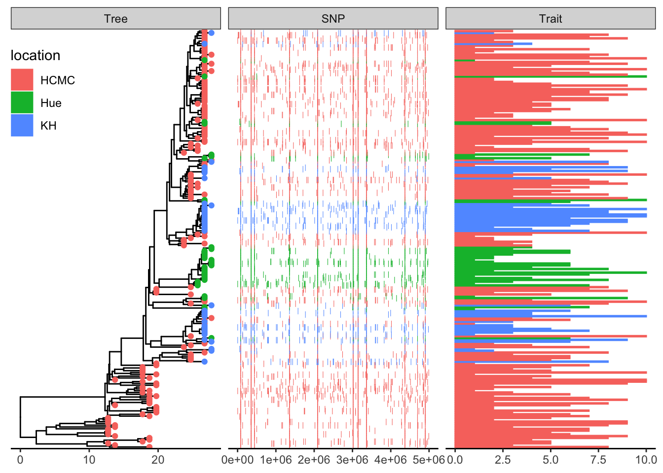
Example datasets
save to your working directory:
bigtree.nex
anolis.SSD.raw.csv
ggtree.R
This is an example of a typical workflow. We have carefully collected phenotypic data, and someone has published a massive phylogeny. We need to subset the tree to just the taxa we want to work on.