Pre-lecture materials

🌴

Read ahead

Before class, you can prepare by reading the following materials:

Acknowledgements

Material for this lecture was borrowed and adopted from

Learning objectives

At the end of this lesson you will:

Understand the tools available to get data into the proper structure and shape for downstream analyses
Learn about the dplyr R package to manage data frames
Recognize the key verbs (functions) to manage data frames in dplyr
Use the “pipe” operator to combine verbs together

Overview

It is still important to understand base R manipulations, particularly for things such as cleaning raw data, troubleshooting, and writing custom functions. But the tidyverse provides many useful tools for data manipuation and analysis of cleaned data. In this session we will learn about dplyr and friends.

Tidy data

The tidyverse has many slogans. A particularly good one for all data analysis is the notion of tidy data.

As defined by Hadley Wickham in his 2014 paper published in the Journal of Statistical Software, a tidy dataset has the following properties:

Each variable forms a column.
Each observation forms a row.
Each type of observational unit forms a table.

[Source: Artwork by Allison Horst]

What shapes does the data need to be in?

Beyond the data being tidy, however, we also need to think about what shape it needs to be in. Weʻll review concepts and tools in the next two lessons.

Now that we have had some experience plotting our data, we can see the value of having rectangular dataframes. We can also see that for particular graphics and analyses, we need to have the data arranged in particular ways.

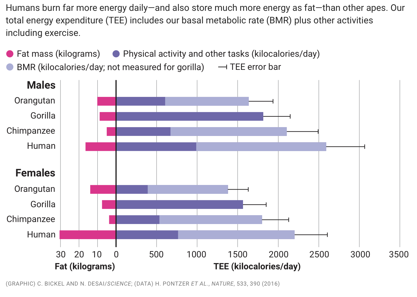
For example, take a look at this elegant graphic below. This single graphic is packed with information on fat, BMR, TEE, and activity levels, all for mulitple species. Is it more effective that individual bar plots? This arrangement is so helpful because you can imagine questions that can be answered with it by comparing the different aspects of the data.

A very informative figure!

Human total energy expenditure compared with other primates. Source: Gibbons, 2022 based on data of H. Ponzer et al., NATURE, 533:90, 2016

Can you imagine what this dataset looks like in terms of organization?

First imagine what it would look like variable by variable.
How might you intially plot the data?
What organization would you need to make a single figure such as this?

We often do not know exactly what we need at the start of a data analysis. We have to play around with different data structures, rearrange the data, look for interesting plots to try, rerrange to fit the input requirements of new functions weʻve discovered, and so on.

Tibbles

The tidyverse uses as its central data structure, the tibble or tbl_df. Tibbles are a variation on data frames, claimed to be lazy and surly:

They don’t change variable names or types when you construct the tibble.
Don’t convert strings to factors (the default behavior in data.frame()).
Complain more when a variable doesnʻt exist.
No row.names() in a tibble. Instead, you must create a new variable.
Display a different summary style for its print() method.
Allows non-standard R names for variables
Allows columns to be lists.

However, most tidyverse functions also work on data frames. Itʻs up to you.

`tibble()` constructor

Just as with data frames, there is a tibble() constructor function, which functions in many ways with similar syntax as the data.frame() constructor.

If you havenʻt already done so, install the tidyverse:

install.packages("tidyverse")

require(tibble)

Loading required package: tibble

tibble( iris[1:4,] )  # the first few rows of iris

# A tibble: 4 × 5
  Sepal.Length Sepal.Width Petal.Length Petal.Width Species
         <dbl>       <dbl>        <dbl>       <dbl> <fct>  
1          5.1         3.5          1.4         0.2 setosa 
2          4.9         3            1.4         0.2 setosa 
3          4.7         3.2          1.3         0.2 setosa 
4          4.6         3.1          1.5         0.2 setosa

x <- 1:3
tibble( x, x * 2 )  # name assigned at construction

# A tibble: 3 × 2
      x `x * 2`
  <int>   <dbl>
1     1       2
2     2       4
3     3       6

silly <- tibble(      # an example of a non-standard names
  `one - 3` = 1:3,  # name = value syntax
  `12` = "numeric",
  `:)` = "smile",
)
silly

# A tibble: 3 × 3
  `one - 3` `12`    `:)` 
      <int> <chr>   <chr>
1         1 numeric smile
2         2 numeric smile
3         3 numeric smile

`as_tibble()` coersion

as_tibble() converts an existing object, such as a data frame or matrix, into a tibble.

as_tibble( iris[1:4,] )  # coercing a dataframe to tibble

# A tibble: 4 × 5
  Sepal.Length Sepal.Width Petal.Length Petal.Width Species
         <dbl>       <dbl>        <dbl>       <dbl> <fct>  
1          5.1         3.5          1.4         0.2 setosa 
2          4.9         3            1.4         0.2 setosa 
3          4.7         3.2          1.3         0.2 setosa 
4          4.6         3.1          1.5         0.2 setosa

As output

Most often we will get tibbles returned from tidyverse functions such as read_csv() from the readr package.

The dplyr package

The dplyr package, which is part of the tidyverse was written to supply a grammar for data manipulation, with verbs for the most common data manipulation tasks.

[Source: Artwork by Allison Horst]

`dplyr` functions

select(): return a subset of the data frame, using a flexible notation
filter(): extract a subset of rows from a data frame using logical conditions
arrange(): reorder rows of a data frame
relocate(): rearrange the columns of a data frame
rename(): rename columns in a data frame
mutate(): add new columns or transform existing variables
summarize(): generate summary statistics of the variables in the data frame, by strata if data are hierarchical
%>%: the “pipe” operator (from magrittr) connects multiple verbs together into a data wrangling pipeline (kind of like making a compound sentence)

Note: Everything dplyr does could already be done with base R. What is different is a new syntax, which allows for more clarity of the data manipulations and the order, and perhaps makes the code more readable.

Instead of the nested syntax, or typing the dataframe name over and over, we can pipe one operation into the next.

Another useful contribution is that dplyr functions are very fast, as many key operations are coded in C++. This will be important for very large datasets or repeated manipulations (say in a simulation study).

`starwars` dataset

We will use the starwars dataset included with dplyr. You should check out the help page for this dataset ?starwars.

Letʻs start by using the skim() function to check out the dataset:

require(dplyr)

Loading required package: dplyr


Attaching package: 'dplyr'

The following objects are masked from 'package:stats':

    filter, lag

The following objects are masked from 'package:base':

    intersect, setdiff, setequal, union

class(starwars)

[1] "tbl_df"     "tbl"        "data.frame"

skimr::skim(starwars)

Data summary
Name	starwars
Number of rows	87
Number of columns	14
_______________________
Column type frequency:
character	8
list	3
numeric	3
________________________
Group variables	None

Variable type: character

skim_variable	n_missing	complete_rate	min	max	n_unique
name	0	1.00	3	21	87
hair_color	5	0.94	4	13	12
skin_color	0	1.00	3	19	31
eye_color	0	1.00	3	13	15
sex	4	0.95	4	14	4
gender	4	0.95	8	9	2
homeworld	10	0.89	4	14	48
species	4	0.95	3	14	37

Variable type: list

skim_variable	complete_rate	n_unique	min_length	max_length
films	1	24	1	7
vehicles	1	11	0	2
starships	1	17	0	5

Variable type: numeric

skim_variable	n_missing	complete_rate	mean	sd	p0	p25	p50	p75	p100	hist
height	6	0.93	174.36	34.77	66	167.0	180	191.0	264	▁▁▇▅▁
mass	28	0.68	97.31	169.46	15	55.6	79	84.5	1358	▇▁▁▁▁
birth_year	44	0.49	87.57	154.69	8	35.0	52	72.0	896	▇▁▁▁▁

Selecting columns with `select()`

Example

Suppose we wanted to take the first 3 columns only. There are a few ways to do this.

We could for example use numerical indices:

names(starwars)[1:3]

[1] "name"   "height" "mass"

But we can also use the names directly:

subset <- select(starwars, c(name, sex:species))
head(subset)

# A tibble: 6 × 5
  name           sex    gender    homeworld species
  <chr>          <chr>  <chr>     <chr>     <chr>  
1 Luke Skywalker male   masculine Tatooine  Human  
2 C-3PO          none   masculine Tatooine  Droid  
3 R2-D2          none   masculine Naboo     Droid  
4 Darth Vader    male   masculine Tatooine  Human  
5 Leia Organa    female feminine  Alderaan  Human  
6 Owen Lars      male   masculine Tatooine  Human

Note

The : normally cannot be used with names or strings, but inside the select() function you can use it to specify a range of variable names.

By exclusion

Variables can be omited using the negative sign withing select():

select( starwars, -(sex:species))

The select() function also has several helper functions that allow matching on patterns. So, for example, if you wanted to keep every variable that ends with “color”:

subset <- select(starwars, ends_with("color"))
str(subset)

tibble [87 × 3] (S3: tbl_df/tbl/data.frame)
 $ hair_color: chr [1:87] "blond" NA NA "none" ...
 $ skin_color: chr [1:87] "fair" "gold" "white, blue" "white" ...
 $ eye_color : chr [1:87] "blue" "yellow" "red" "yellow" ...

Or all variables that start with n or m:

subset <- select(starwars, starts_with("n") | starts_with("m"))
str(subset)

tibble [87 × 2] (S3: tbl_df/tbl/data.frame)
 $ name: chr [1:87] "Luke Skywalker" "C-3PO" "R2-D2" "Darth Vader" ...
 $ mass: num [1:87] 77 75 32 136 49 120 75 32 84 77 ...

You can also use more general regular expressions. See the help page (?select) for more details.

Subsetting with `filter()`

The filter() function is used to extract subsets of rows or observations from a data frame. This function is similar to the existing subset() function in base R, or indexing by logical comparisons.

Artwork by Allison Horst on filter() function

[Source: Artwork by Allison Horst]

Example

Suppose we wanted to extract the rows of the starwars data frame where the birthyear is greater than 100:

age100 <- filter(starwars, birth_year > 100)
head(age100)

# A tibble: 5 × 14
  name      height  mass hair_color skin_color eye_color birth_year sex   gender
  <chr>      <int> <dbl> <chr>      <chr>      <chr>          <dbl> <chr> <chr> 
1 C-3PO        167    75 <NA>       gold       yellow           112 none  mascu…
2 Chewbacca    228   112 brown      unknown    blue             200 male  mascu…
3 Jabba De…    175  1358 <NA>       green-tan… orange           600 herm… mascu…
4 Yoda          66    17 white      green      brown            896 male  mascu…
5 Dooku        193    80 white      fair       brown            102 male  mascu…
# ℹ 5 more variables: homeworld <chr>, species <chr>, films <list>,
#   vehicles <list>, starships <list>

You can see that there are now only 5 rows in the data frame and the distribution of the birth_year values is.

summary(age100$birth_year)

   Min. 1st Qu.  Median    Mean 3rd Qu.    Max. 
    102     112     200     382     600     896

We can also filter on multiple conditions: and requires both conditions to be true, whereas or requires only one to be true. This time letʻs choose birth_year < 100 and homeworld == "Tatooine:

age_tat <- filter(starwars, birth_year < 100 & homeworld == "Tatooine")
select(age_tat, name, height, mass, birth_year, sex)

# A tibble: 8 × 5
  name               height  mass birth_year sex   
  <chr>               <int> <dbl>      <dbl> <chr> 
1 Luke Skywalker        172    77       19   male  
2 Darth Vader           202   136       41.9 male  
3 Owen Lars             178   120       52   male  
4 Beru Whitesun lars    165    75       47   female
5 Biggs Darklighter     183    84       24   male  
6 Anakin Skywalker      188    84       41.9 male  
7 Shmi Skywalker        163    NA       72   female
8 Cliegg Lars           183    NA       82   male

Other logical operators you should be aware of include:

Operator	Meaning	Example
`==`	Equals	`homeworld == Tatooine`
`!=`	Does not equal	`homeworld != Tatooine`
`>`	Greater than	`height > 170.0`
`>=`	Greater than or equal to	`height >= 170.0`
`<`	Less than	`height < 170.0`
`<=`	Less than or equal to	`height <= 170.0`
`%in%`	Included in	`homeworld %in% c("Tatooine", "Naboo")`
`is.na()`	Is a missing value	`is.na(mass)`

Note

If you are ever unsure of how to write a logical statement, but know how to write its opposite, you can use the ! operator to negate the whole statement.

A common use of this is to identify observations with non-missing data (e.g., !(is.na(homweworld))).

Sorting data with `arrange()`

arrange() is like the sort function in a spreadsheet, or order() in base R. arrange() reorders rows of a data frame according to one of the columns. Think of this as sorting your rows on the value of a column.

Here we can order the rows of the data frame by birth_year, so that the first row is the earliest (oldest) observation and the last row is the latest (most recent) observation.

starwars <- arrange(starwars, birth_year)

We can now check the first few rows

head(select(starwars, name, birth_year), 3)

# A tibble: 3 × 2
  name                  birth_year
  <chr>                      <dbl>
1 Wicket Systri Warrick          8
2 IG-88                         15
3 Luke Skywalker                19

and the last few rows.

tail(select(starwars, name, birth_year), 3)

# A tibble: 3 × 2
  name           birth_year
  <chr>               <dbl>
1 Poe Dameron            NA
2 BB8                    NA
3 Captain Phasma         NA

Columns can be arranged in descending order using the helper function desc().

starwars <- arrange(starwars, desc(birth_year))

Looking at the first three and last three rows shows the dates in descending order.

head(select(starwars, name, birth_year), 3)

# A tibble: 3 × 2
  name                  birth_year
  <chr>                      <dbl>
1 Yoda                         896
2 Jabba Desilijic Tiure        600
3 Chewbacca                    200

tail(select(starwars, name, birth_year), 3)

# A tibble: 3 × 2
  name           birth_year
  <chr>               <dbl>
1 Poe Dameron            NA
2 BB8                    NA
3 Captain Phasma         NA

Rearranging columns with `relocate()`

Moving a column to a new location is done by specifying the column names, and indicating where they go with the .before= or .after= arguments specifing a location (another column).

relocate(.data, ..., .before = NULL, .after = NULL)

Renaming columns with `rename()`

Renaming a variable in a data frame in R is accomplished using the names() function. The rename() function is designed to make this process easier.

Here you can see the names of the first six variables in the starwars data frame.

head(starwars[, 1:6], 3)

# A tibble: 3 × 6
  name                  height  mass hair_color skin_color       eye_color
  <chr>                  <int> <dbl> <chr>      <chr>            <chr>    
1 Yoda                      66    17 white      green            brown    
2 Jabba Desilijic Tiure    175  1358 <NA>       green-tan, brown orange   
3 Chewbacca                228   112 brown      unknown          blue

Suppose we wanted to drop the _color. The syntax is newname = oldname:

starwars <- rename(starwars, hair = hair_color, skin = skin_color, eye = eye_color)
head(starwars[, 1:6], 3)

# A tibble: 3 × 6
  name                  height  mass hair  skin             eye   
  <chr>                  <int> <dbl> <chr> <chr>            <chr> 
1 Yoda                      66    17 white green            brown 
2 Jabba Desilijic Tiure    175  1358 <NA>  green-tan, brown orange
3 Chewbacca                228   112 brown unknown          blue

Question

How would you do the equivalent in base R without dplyr?

Adding columns with `mutate()`

The mutate() function computes transformations of variables in a data frame.

Artwork by Allison Horst on mutate() function

[Source: Artwork by Allison Horst]

For example, we may want to adjust height for mass:

starwars <- mutate(starwars, heightsize = height / mass )
head(starwars)

# A tibble: 6 × 15
  name  height  mass hair  skin  eye   birth_year sex   gender homeworld species
  <chr>  <int> <dbl> <chr> <chr> <chr>      <dbl> <chr> <chr>  <chr>     <chr>  
1 Yoda      66    17 white green brown        896 male  mascu… <NA>      Yoda's…
2 Jabb…    175  1358 <NA>  gree… oran…        600 herm… mascu… Nal Hutta Hutt   
3 Chew…    228   112 brown unkn… blue         200 male  mascu… Kashyyyk  Wookiee
4 C-3PO    167    75 <NA>  gold  yell…        112 none  mascu… Tatooine  Droid  
5 Dooku    193    80 white fair  brown        102 male  mascu… Serenno   Human  
6 Qui-…    193    89 brown fair  blue          92 male  mascu… <NA>      Human  
# ℹ 4 more variables: films <list>, vehicles <list>, starships <list>,
#   heightsize <dbl>

There is also the related transmute() function, which mutate()s and keeps only the transformed variables. Therefore, the result is only two columns in the transmuted data frame.

Perform functions on groups using `group_by()`

The group_by() function is used to indicate groups within the data.

For example, what is the average height by homeworld?

In conjunction with the group_by() function, we often use the summarize() function.

Note

The general operation here is a combination of

Splitting a data frame by group defined by a variable or group of variables (group_by())
summarize() across those subsets

Example

We can create a separate data frame that splits the original data frame by homeworld.

worlds <- group_by(starwars, homeworld)

Compute summary statistics by planet (just showing mean and median here, almost any summary stat is available):

summarize(worlds, height = mean(height, na.rm = TRUE), 
          maxheight = max(height, na.rm = TRUE),
          mass = median(mass, na.rm = TRUE))

# A tibble: 49 × 4
   homeworld      height maxheight  mass
   <chr>           <dbl>     <dbl> <dbl>
 1 Alderaan         176.      176.  64  
 2 Aleen Minor       79        79   15  
 3 Bespin           175       175   79  
 4 Bestine IV       180       180  110  
 5 Cato Neimoidia   191       191   90  
 6 Cerea            198       198   82  
 7 Champala         196       196   NA  
 8 Chandrila        150       150   NA  
 9 Concord Dawn     183       183   79  
10 Corellia         175       175   78.5
# ℹ 39 more rows

summarize() returns a data frame with homeworld as the first column, followed by the requested summary statistics. This is similar to the base R function aggregate().

More complicated example

In a slightly more complicated example, we might want to know what are the average masses within quintiles of height:

First, we can create a categorical variable of height5 divided into quintiles

qq <- quantile(starwars$height, seq(0, 1, 0.2), na.rm = TRUE)
starwars <- mutate(starwars, height.quint = cut(height, qq))

Now we can group the data frame by the height.quint variable.

quint <- group_by(starwars, height.quint)

Finally, we can compute the mean of mass within quintiles of height.

summarize(quint, mquint = mean(mass, na.rm = TRUE))

# A tibble: 6 × 2
  height.quint mquint
  <fct>         <dbl>
1 (66,165]       44.2
2 (165,175]     187. 
3 (175,183]      79.2
4 (183,193]      80.2
5 (193,264]     106. 
6 <NA>           17

Oddly enough there is a maximum mass in the second height quintile of Starwars characters. The biologist in me thinks maybe outliers?

Piping multiple functions using `%>%`

The pipe operator %>% is very handy for stringing together multiple dplyr functions in a sequence of operations. It comes from the magritter package.

Source:

In base R, there are two styles of applying multiple functions. The first is the resave the object after each operation.

The second is to nest functions, with the first at the deepest level (the heart of the onion), then working our way out:

third(second(first(x)))

The %>% operator allows you to string operations in a left-to-right fashion, where the output of one flows into the next, i.e.:

first(x) %>% second %>% third

Example

Take the example that we just did in the last section.

That can be done with the following sequence:

starwars %>% 
  group_by(homeworld) %>% 
  summarize(height = mean(height, na.rm = TRUE), 
          maxheight = max(height, na.rm = TRUE),
          mass = median(mass, na.rm = TRUE))

# A tibble: 49 × 4
   homeworld      height maxheight  mass
   <chr>           <dbl>     <dbl> <dbl>
 1 Alderaan         176.      176.  64  
 2 Aleen Minor       79        79   15  
 3 Bespin           175       175   79  
 4 Bestine IV       180       180  110  
 5 Cato Neimoidia   191       191   90  
 6 Cerea            198       198   82  
 7 Champala         196       196   NA  
 8 Chandrila        150       150   NA  
 9 Concord Dawn     183       183   79  
10 Corellia         175       175   78.5
# ℹ 39 more rows

Data masking

Notice that we did not have to specify the dataframe. This is because dplyr functions are built on a data masking syntax. From the dplyr data-masking help page:

Data masking allows you to refer to variables in the “current” data frame (usually supplied in the .data argument), without any other prefix. It’s what allows you to type (e.g.) filter(diamonds, x == 0 & y == 0 & z == 0) instead of diamonds[diamonds$x == 0 & diamonds$y == 0 & diamonds$z == 0, ]

When you look at the help page for ?mutate for example, you will see a function definition like so:

mutate(.data, ...)

Note the .data, Which means that the data can be supplied as usual, or it can be inherited from the “current” data frame which is passed to it via a pipe.

Sample rows of data with `slice_*()`

The slice_sample() function will randomly sample rows of data.

The number of rows to show is specified by the n argument.

This can be useful if you do not want to print the entire tibble, but you want to get a greater sense of the variation.

Example

slice_sample(starwars, n = 10)

# A tibble: 10 × 16
   name         height  mass hair  skin  eye   birth_year sex   gender homeworld
   <chr>         <int> <dbl> <chr> <chr> <chr>      <dbl> <chr> <chr>  <chr>    
 1 Darth Vader     202   136 none  white yell…       41.9 male  mascu… Tatooine 
 2 San Hill        191    NA none  grey  gold        NA   male  mascu… Muunilin…
 3 Bail Presto…    191    NA black tan   brown       67   male  mascu… Alderaan 
 4 Mon Mothma      150    NA aubu… fair  blue        48   fema… femin… Chandrila
 5 Zam Wesell      168    55 blon… fair… yell…       NA   fema… femin… Zolan    
 6 Anakin Skyw…    188    84 blond fair  blue        41.9 male  mascu… Tatooine 
 7 Cliegg Lars     183    NA brown fair  blue        82   male  mascu… Tatooine 
 8 Sebulba         112    40 none  grey… oran…       NA   male  mascu… Malastare
 9 Quarsh Pana…    183    NA black dark  brown       62   <NA>  <NA>   Naboo    
10 Gregar Typho    185    85 black dark  brown       NA   male  mascu… Naboo    
# ℹ 6 more variables: species <chr>, films <list>, vehicles <list>,
#   starships <list>, heightsize <dbl>, height.quint <fct>

You can also use slice_head() or slice_tail() to take a look at the top rows or bottom rows of your tibble. Again the number of rows can be specified with the n argument.

This will show the first 5 rows.

slice_head(starwars, n = 5)

# A tibble: 5 × 16
  name  height  mass hair  skin  eye   birth_year sex   gender homeworld species
  <chr>  <int> <dbl> <chr> <chr> <chr>      <dbl> <chr> <chr>  <chr>     <chr>  
1 Yoda      66    17 white green brown        896 male  mascu… <NA>      Yoda's…
2 Jabb…    175  1358 <NA>  gree… oran…        600 herm… mascu… Nal Hutta Hutt   
3 Chew…    228   112 brown unkn… blue         200 male  mascu… Kashyyyk  Wookiee
4 C-3PO    167    75 <NA>  gold  yell…        112 none  mascu… Tatooine  Droid  
5 Dooku    193    80 white fair  brown        102 male  mascu… Serenno   Human  
# ℹ 5 more variables: films <list>, vehicles <list>, starships <list>,
#   heightsize <dbl>, height.quint <fct>

This will show the last 5 rows.

slice_tail(starwars, n = 5)

# A tibble: 5 × 16
  name  height  mass hair  skin  eye   birth_year sex   gender homeworld species
  <chr>  <int> <dbl> <chr> <chr> <chr>      <dbl> <chr> <chr>  <chr>     <chr>  
1 Finn      NA    NA black dark  dark          NA male  mascu… <NA>      Human  
2 Rey       NA    NA brown light hazel         NA fema… femin… <NA>      Human  
3 Poe …     NA    NA brown light brown         NA male  mascu… <NA>      Human  
4 BB8       NA    NA none  none  black         NA none  mascu… <NA>      Droid  
5 Capt…     NA    NA unkn… unkn… unkn…         NA <NA>  <NA>   <NA>      <NA>   
# ℹ 5 more variables: films <list>, vehicles <list>, starships <list>,
#   heightsize <dbl>, height.quint <fct>

Summary

The dplyr package provides an alternative syntax for manipulating data frames. In particular, we can often conduct the beginnings of an exploratory analysis with the powerful combination of group_by() and summarize().

Once you learn the dplyr grammar there are a few additional benefits

dplyr can work with other data frame “back ends” such as SQL databases. There is an SQL interface for relational databases via the DBI package
dplyr can be integrated with the data.table package for large fast tables
Many people like the piping syntax for readability and clarity

Post-lecture materials

Final Questions

Questions

How can you tell if an object is a tibble?
Using the trees dataset in base R (this dataset stores the girth, height, and volume for Black Cherry Trees) and using the pipe operator:
1. convert the data.frame to a tibble.
2. filter for rows with a tree height of greater than 70, and
3. order rows by Volume (smallest to largest).

head(trees)

  Girth Height Volume
1   8.3     70   10.3
2   8.6     65   10.3
3   8.8     63   10.2
4  10.5     72   16.4
5  10.7     81   18.8
6  10.8     83   19.7

Additional Resources

Tip

Pre-lecture materials

Read ahead

Acknowledgements

Learning objectives

Overview

Tidy data

What shapes does the data need to be in?

Tibbles

tibble() constructor

as_tibble() coersion

As output

The dplyr package

dplyr functions

starwars dataset

Selecting columns with select()

By exclusion

Subsetting with filter()

Sorting data with arrange()

Rearranging columns with relocate()

Renaming columns with rename()

Adding columns with mutate()

Perform functions on groups using group_by()

Piping multiple functions using %>%

Data masking

Sample rows of data with slice_*()

Summary

Post-lecture materials

Final Questions

Additional Resources

`tibble()` constructor

`as_tibble()` coersion

`dplyr` functions

`starwars` dataset

Selecting columns with `select()`

Subsetting with `filter()`

Sorting data with `arrange()`

Rearranging columns with `relocate()`

Renaming columns with `rename()`

Adding columns with `mutate()`

Perform functions on groups using `group_by()`

Piping multiple functions using `%>%`

Sample rows of data with `slice_*()`