install.packages("gapminder") # a dataset packagePre-lecture materials
Read ahead
Read ahead
Before class, you can prepare by reading the following materials:
Acknowledgements
Material for this lecture was borrowed and adopted from
Learning objectives
Learning objectives
At the end of this lesson you will:
- Be able to define relational data and keys
- Be able to define the three types of join functions for relational data
- Be able to implement mutational join functions
New Packages
You will have to install if you donʻt already have them:
Overview
Last time we talked about tidy data. One common issue is that people sometimes use column names to store data. For example take a look at this built-in dataset that comes with tidyr on religion and income survey data with the number of respondents with income range in column name.
Joining data (a.k.a. Merging)
Relational data
Data analyses rarely involve only a single table of data.
Typically you have many tables of data, and you must combine the datasets to answer the questions that you are interested in. Some examples include morphology and ecology data on the same species, or sequence data and metadata.
Collectively, multiple tables of data are called relational data because it is the relations, not just the individual datasets, that are important.
Relations are always defined between a pair of tables. All other relations are built up from this simple idea: the relations of three or more tables are always a property of the relations between each pair.
Sometimes both elements of a pair can be in the same table! This is needed if, for example, you have a table of people, and each person has a reference to their parents, or if you have nodes in a phylogeny and each is linked to an ancestral node.
Relational data are combined with merges or joins.
Example with merge()
Letʻs use the geospiza data from the geiger package to practice merging with the base R merge() function.
require(geiger)
data(geospiza)   # load the dataset into the workspace
ls()               # list the objects in the workspace
[1] "geospiza"geospiza$geospiza.tree
Phylogenetic tree with 14 tips and 13 internal nodes.
Tip labels:
fuliginosa, fortis, magnirostris, conirostris, scandens, difficilis, ...
Rooted; includes branch lengths.
$geospiza.data
wingL tarsusL culmenL beakD gonysW
magnirostris 4.404200 3.038950 2.724667 2.823767 2.675983
conirostris 4.349867 2.984200 2.654400 2.513800 2.360167
difficilis 4.224067 2.898917 2.277183 2.011100 1.929983
scandens 4.261222 2.929033 2.621789 2.144700 2.036944
fortis 4.244008 2.894717 2.407025 2.362658 2.221867
fuliginosa 4.132957 2.806514 2.094971 1.941157 1.845379
pallida 4.265425 3.089450 2.430250 2.016350 1.949125
fusca 3.975393 2.936536 2.051843 1.191264 1.401186
parvulus 4.131600 2.973060 1.974420 1.873540 1.813340
pauper 4.232500 3.035900 2.187000 2.073400 1.962100
Pinaroloxias 4.188600 2.980200 2.311100 1.547500 1.630100
Platyspiza 4.419686 3.270543 2.331471 2.347471 2.282443
psittacula 4.235020 3.049120 2.259640 2.230040 2.073940
$phy
Phylogenetic tree with 14 tips and 13 internal nodes.
Tip labels:
fuliginosa, fortis, magnirostris, conirostris, scandens, difficilis, ...
Rooted; includes branch lengths.
$dat
wingL tarsusL culmenL beakD gonysW
magnirostris 4.404200 3.038950 2.724667 2.823767 2.675983
conirostris 4.349867 2.984200 2.654400 2.513800 2.360167
difficilis 4.224067 2.898917 2.277183 2.011100 1.929983
scandens 4.261222 2.929033 2.621789 2.144700 2.036944
fortis 4.244008 2.894717 2.407025 2.362658 2.221867
fuliginosa 4.132957 2.806514 2.094971 1.941157 1.845379
pallida 4.265425 3.089450 2.430250 2.016350 1.949125
fusca 3.975393 2.936536 2.051843 1.191264 1.401186
parvulus 4.131600 2.973060 1.974420 1.873540 1.813340
pauper 4.232500 3.035900 2.187000 2.073400 1.962100
Pinaroloxias 4.188600 2.980200 2.311100 1.547500 1.630100
Platyspiza 4.419686 3.270543 2.331471 2.347471 2.282443
psittacula 4.235020 3.049120 2.259640 2.230040 2.073940geo <- geospiza$dat # save the morphometric data as geoThis is a 5 column dataframe. Letʻs take just the tarsusL data to build our example dataset:
tarsusL <- geo[,"tarsusL"]  # geo is a matrix, select tarsusL column
geot <- data.frame(tarsusL, "ecology" = LETTERS[1:length(tarsusL)])
Often we will be merging data that donʻt perfectly match. Some parts of the data will be missing, for example we may only have ecology data for the first five species. The question is what do you want the merge behavior to be?
The default is to drop all observations that are not in BOTH datasets. Here we merge the original geo with only the first five rows of geot:
                    # only maches to both datasets are included
merge(x=geo[,"tarsusL"], y=geot[1:5, ], by= "row.names")
Row.names x tarsusL ecology
1 conirostris 2.984200 2.984200 B
2 difficilis 2.898917 2.898917 C
3 fortis 2.894717 2.894717 E
4 magnirostris 3.038950 3.038950 A
5 scandens 2.929033 2.929033 DIf we want to keep everything, use the all=T flag:
                    # all species in both datasets are included
merge(x=geo[,"tarsusL"], y=geot[1:5,], by= "row.names", all=T)
Row.names x tarsusL ecology
1 conirostris 2.984200 2.984200 B
2 difficilis 2.898917 2.898917 C
3 fortis 2.894717 2.894717 E
4 fuliginosa 2.806514 NA <NA>
5 fusca 2.936536 NA <NA>
6 magnirostris 3.038950 3.038950 A
7 pallida 3.089450 NA <NA>
8 parvulus 2.973060 NA <NA>
9 pauper 3.035900 NA <NA>
10 Pinaroloxias 2.980200 NA <NA>
11 Platyspiza 3.270543 NA <NA>
12 psittacula 3.049120 NA <NA>
13 scandens 2.929033 2.929033 DThere is also all.x which keeps all values of the first data table but drops non-matching rows of the second table, and all.y which keeps all of the second.
The results of merge are sorted by default on the sort key. To turn it off:
geo <- geo[rev(rownames(geo)), ]   # reverse the species order of geo
                     # merge on geo first, then geot
merge(x=geo[,"tarsusL"], y=geot[1:5, ], by= "row.names", sort=F)
Row.names x tarsusL ecology
1 fortis 2.894717 2.894717 E
2 scandens 2.929033 2.929033 D
3 difficilis 2.898917 2.898917 C
4 conirostris 2.984200 2.984200 B
5 magnirostris 3.038950 3.038950 A # geot first, then geo
merge(x=geot[1:5,], y=geo[,"tarsusL"], by= "row.names", sort=F) Row.names tarsusL ecology y
1 magnirostris 3.038950 A 3.038950
2 conirostris 2.984200 B 2.984200
3 difficilis 2.898917 C 2.898917
4 scandens 2.929033 D 2.929033
5 fortis 2.894717 E 2.894717
Note
- In a
merge, the non-key columns are copied over into the new table.
Check out the help page for ?merge for more info.
Keys
The variables used to connect each pair of tables are called keys. A key is a variable (or set of variables) that uniquely identifies an observation. In simple cases, a single variable is sufficient to identify an observation.
In the example above the key was the species names, which was contained in the row.names attribute. The key was specified in the merge in the by= argument. A merge or join key is a generic concept that is used in many database operations.
Note
There are two types of keys:
- A primary key uniquely identifies an observation in its own table.
- A foreign key uniquely identifies an observation in another table.
Let’s consider an example to help us understand the difference between a primary key and foreign key.
Example of keys
Imagine you are conduct a study and collecting data on subjects and a health outcome.
Often, subjects will have multiple observations (a longitudinal study). Similarly, we may record other information, such as the type of housing.
The first table
This code creates a simple table with some made up data about some hypothetical subjects’ outcomes.
library(tidyverse)

outcomes <- tibble(
        id = rep(c("a", "b", "c"), each = 3),
        visit = rep(0:2, 3),
        outcome = rnorm(3 * 3, 3)
)

print(outcomes)
# A tibble: 9 × 3
id visit outcome
<chr> <int> <dbl>
1 a 0 4.41
2 a 1 1.55
3 a 2 3.73
4 b 0 4.40
5 b 1 3.13
6 b 2 3.77
7 c 0 2.43
8 c 1 2.09
9 c 2 3.17Note that subjects are labeled by a unique identifer in the id column.
A second table
Here is some code to create a second table containing data about the hypothetical subjects’ housing type.
subjects <- tibble(
        id = c("a", "b", "c"),
        house = c("detached", "rowhouse", "rowhouse")
)

print(subjects)
# A tibble: 3 × 2
id house
<chr> <chr>
1 a detached
2 b rowhouse
3 c rowhouse
Question
What is the primary key and foreign key?
- The
outcomes$idis a primary key because it uniquely identifies each subject in theoutcomestable. - The
subjects$idis a foreign key because it appears in thesubjectstable where it matches each subject to a uniqueid.
Joining in dplyr
In dplyr, merges are called joins (both are used in database science) and introduces a vocabulary that names each of these situations.
Three important families of joins
-
Mutating joins: add new variables to one data frame from matching observations in another.
- This is a typical merge operation. A mutating join combines variables from two tables into a new table. Observations in the two tables are matched by their keys, with the variables from the two tables copied into the new table. It is a mutating join because it adds columns with the merge, and in that way is analogous to the
mutate()function for dataframes.
- See Section 7 for Table of mutating joins.
- This is a typical merge operation. A mutating join combines variables from two tables into a new table. Observations in the two tables are matched by their keys, with the variables from the two tables copied into the new table. It is a mutating join because it adds columns with the merge, and in that way is analogous to the
-
Filtering joins: filter observations from one data frame based on whether or not they match an observation in the other table
- Filtering joins are a way to filter one dataset by observations in another dataset (they are more filter and less join).
- Filtering joins match observations by a key, as usual, but select the observations that match (not the variables). In other words, this type of join filters observations from one data frame based on whether or not they match an observation in the other.
- Two types:
semi_join(x, y)andanti_join(x, y).
-
Set operations: treat observations as if they were set elements.
- Set operations can be useful when you want to break a single complex filter into simpler pieces. All these operations work with a complete row, comparing the values of every variable. These expect the x and y inputs to have the same variables, and treat the observations like sets:
- Examples of set operations:
intersect(x, y),union(x, y), andsetdiff(x, y).
- Set operations can be useful when you want to break a single complex filter into simpler pieces. All these operations work with a complete row, comparing the values of every variable. These expect the x and y inputs to have the same variables, and treat the observations like sets:
Types of mutating joins
The dplyr package provides a set of functions for joining two data frames into a single data frame based on a set of key columns.
There are several functions in the *_join() family.
- These functions all merge together two data frames
- They differ in how they handle observations that exist in one but not both data frames.
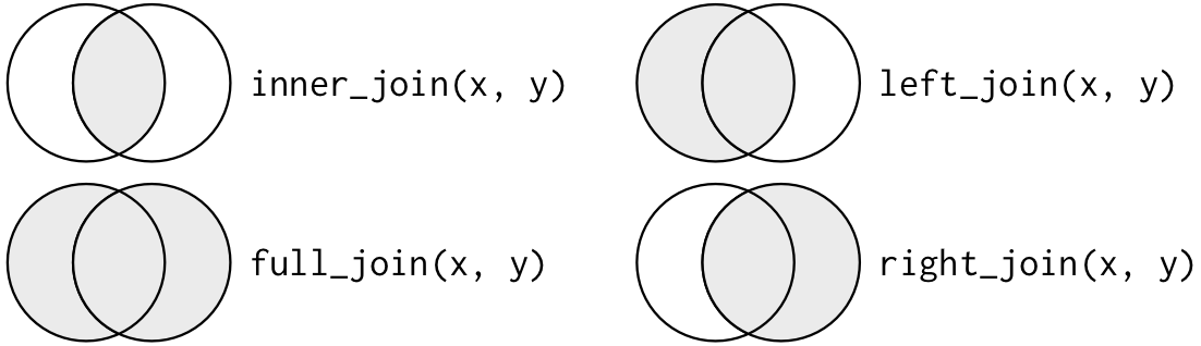
Here, are the four functions from this family that you will likely use the most often:
| Function | What it includes in merged data frame |
|---|---|
left_join() |
Includes all observations in the left data frame, whether or not there is a match in the right data frame |
right_join() |
Includes all observations in the right data frame, whether or not there is a match in the left data frame |
inner_join() |
Includes only observations that are in both data frames |
full_join() |
Includes all observations from both data frames |
Post-lecture materials
Final Questions
Here are some post-lecture questions to help you think about the material discussed.
Questions
Using prose, describe how the variables and observations are organised in a tidy dataset versus an non-tidy dataset.
What do the extra and fill arguments do in
separate()? Experiment with the various options for the following two toy datasets.
Both
unite()andseparate()have a remove argument. What does it do? Why would you set it to FALSE?Compare and contrast
separate()andextract(). Why are there three variations of separation (by position, by separator, and with groups), but only oneunite()?