Acknowledgements

Material for this lecture was borrowed and adopted from

https://www.r-bloggers.com/2015/04/tips-tricks-8-examining-replicate-error/

Learning objectives

At the end of this lesson you will:

Be able to estimate measurement error and repeatability

Overview

Measurement Error and Repeatability

Morphometrics is all about assessing variability, within and between individuals. One of those sources of variability is measurement error.

Measurement Error (ME) itself comes from many potential sources:

the measurement device (precision)
definition of the measure
quality of the measured material
the measurer
the environment of the measurer (hopefully small!)
measurement protocol

We try to minimize ME so that we can reveal the underlying patterns we are interested in, but there will always be some ME. So it is important to quantify at least once at the beginning of the study.

Protocol for assessing ME

The percentage of measurement error is defined as the within-group component of variance divided by the total (within + betwee group) variance (Claude 2008):

\[ \%ME = \frac{s^{2}_{within}}{s^{2}_{within} + s^{2}_{among}} \times 100 \]

We can get the componets of variance \(s^{2}\) from the mean squares (\(MSS\)) of an ANOVA considering the individual (as a factor) source of variation. Individual here represents the within-group variation. The among and within variance can be estimated from the mean sum of squares and \(m\) the number of repeated measurements:

\[ s^{2}_{among} = \frac{MSS_{among} - MSS_{within}}{m} \]

and

\[ s^{2}_{within} = MSS_{within} \]

Example

Let’s say you are taking photographs of your specimens and you want to quantify the error assocated with placing your landmarks in the same place every time (i.e. is your criteria for the landmark robust enough that its obvious where it should be placed on each specimen, and if you came back to the data a month or year later?)

To assess measurement error in this instance we could take two sets of pictures, each time removing and positioning the specimen. And we could digitize each image twice, preferably in different sessions (another day or week). This would give us 4 sets of landmark data for each specimen, allowing us to asses both error associated with the digitization as well as error in capturing the shapes via the photographs.

Alternatively, if we were interested in inter-observer error vs. repeatability within observer, we could take one photograph and have it measured by two different people, each person taking two sets of measurements (preferably in different sessions).

Simulated example:

Repeat a set of five measurements, (measure twice), once in each of two sessions on different days. How repeatable are the measurements?

Simulate the data:

true_m <- rnorm(5,20,3)  # true values
m1 <- true_m + rnorm(5,0,1) # measurements set 1
m2 <- true_m + rnorm(5,0,1)
session <- gl(2, 5)
individual <- as.factor(rep(1:5,2))
total_m <- c(m1, m2)
cbind(individual, total_m, session)  # the data

      individual  total_m session
 [1,]          1 20.44919       1
 [2,]          2 21.85592       1
 [3,]          3 23.57399       1
 [4,]          4 23.66764       1
 [5,]          5 15.82221       1
 [6,]          1 20.61579       2
 [7,]          2 22.73522       2
 [8,]          3 22.57645       2
 [9,]          4 23.67244       2
[10,]          5 13.60084       2

summary(aov(total_m ~ session))

            Df Sum Sq Mean Sq F value Pr(>F)
session      1   0.47    0.47   0.035  0.857
Residuals    8 108.45   13.56

There is no difference between sessions (yay)!

mod <- summary(aov(total_m ~ individual))
mod

            Df Sum Sq Mean Sq F value   Pr(>F)    
individual   4 105.55  26.388   39.21 0.000574 ***
Residuals    5   3.37   0.673                     
---
Signif. codes:  0 '***' 0.001 '**' 0.01 '*' 0.05 '.' 0.1 ' ' 1

The specimens measured (individuals) are significantly different.

s2within <- MSwithin <- mod[[1]][2,3]
MSamong <- mod[[1]][1,3]
s2among <- (MSamong-MSwithin)/2
pME <- s2within/(s2within+s2among)*100
pME

[1] 4.974382

And the percent measurement error is represented by pME. As a rough rule of thumb we want this to be less than 5%. If it is very high, we either want to practice more, or take multiple measurements of each variable and average them.

Calculating morphometric parameters

Your raw data may be in lengths for linear morphometrics or coordinate for landmark-based morphometrics. You will often have to calcuate quantities from your raw data such as distances and angles.

Calculating distances

You may need to calculate distances between your landmarks, or you may have species centroids (the means in multiple dimensions), and you want to know the distance between species in morphospace.

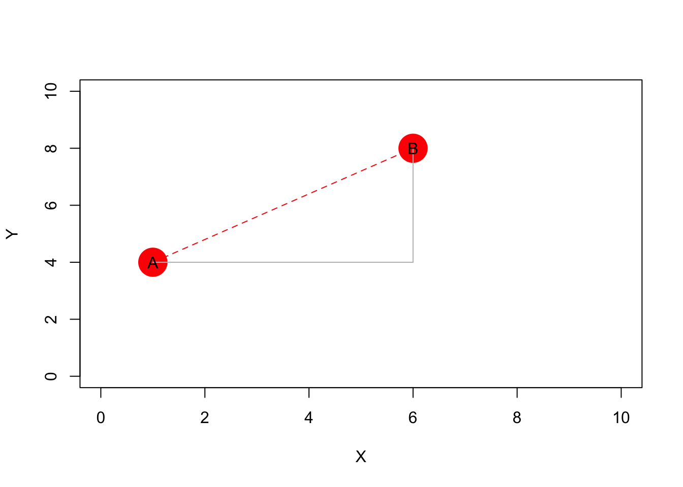
The distance between two points (in k dimensions) is given by the square root of the sum of the squared differences between the points.

\[ d_{AB} = \sqrt{\sum_{i=1}^{k}} (A_i - B_i)^2 \]

This is analogous to calcuating the length of the hypotenuse in a right triangle. If there is more than one dimension, these squared differences are computed dimension by dimension, summed, then the entire quantity is square rooted.

A 2-D example in R is:

A <- c(1,4)
B <- c(6,8)
plot( c(A[1], B[1]),c(A[2], B[2]), xlim=c(0,10), ylim=c(0,10), 
      xlab="X", ylab="Y", cex=4,  pch=16, col="red")
lines( c(A[1], B[1]),c(A[2], B[2]), lty=2, col="red" )
lines( c(A[1], B[1]),c(A[2], A[2]), col="grey" )
lines( c(B[1], B[1]),c(A[2], B[2]), col="grey" )
text(A[1], A[2], "A")
text(B[1], B[2], "B")

Compute the distance:

A-B

[1] -5 -4

sum((A-B)^2)

[1] 41

sqrt(sum((A-B)^2))

[1] 6.403124

We can create a function:

distance <- function( A, B ) { sqrt(sum((A-B)^2)) }
distance( A, B )

[1] 6.403124

Try it on a 3-D set of coordinates. Does it work?

Angle between two vectors

The angle \(\theta\) between two vectors \(\overrightarrow{AB}\) and \(\overrightarrow{CD}\) can be calculated using the dot product and the rule of cosines.

Suppose we have two vectors \(V_1 = (x_1,y_1)\), and \(V2 = (x_2,y_2)\). We can use our coordinates A, B above to calculate our first vector, and make up a second one. From geometry, we can think of vectors as originating at (0,0) with the vector coordinates indicating the head of the vector.

V1 <- AB <- B - A  # using our A,B landmarks above
V1

[1] 5 4

V2 <- c(2,4)  # another vector

The dot product is then:

\[ V_1V_2 = x_1x_2 + y_1y_2 = |V_1| \cdot |V_2| cos(\theta) \]

Rearranging:

\[ cos(\theta) = \frac{ x_1x_2 + y_1y_2 } { |V_1| \cdot |V_2| } \]

Also \[ |V_1| = \sqrt{ x_1^2 + y_1^2} \]

And similarly for \(V_2\).

So all we have to do is take the inverse cosine, arc cosine, or acos() to solve for the angle theta (\(\theta\)).

Calculating the angle in R

V1 %*% V2  # the dot product. what is the difference with V1 * V2?

     [,1]
[1,]   26

           # same as sum(V1*V2) 

theta <- acos( (V1 %*% V2) / (sqrt( V1%*%V1) * sqrt(V2%*%V2)) )
theta

          [,1]
[1,] 0.4324078

Where the result is in radians, not degrees (see the help page ?acos, all of Rʻs trig functions are in radians).

Note: I should change this to using the arc tangent, to preserve the angle in case it is outside of 0,pi.

Radians to degrees

Degrees and radians are different units of measure for an angle. To covert to degrees, remember that a 360 degree circle is 2pi radians (or a half circle 180 degrees is pi radians):

To remember how to do this conversion, recall that the formula for the circumference of a circle is:

\[ Circumference = 2 \pi r \]

A few key facts:

Arc length : the distance along a curved line (the arc length of the entire circle is the circumference).
Radian : the angle measured in relation to the radius. If you take the radius and lay it along the circle, the angle defined by the arc length of one radius is one radian.
To complete the circle, we need an arc length of \(2\pi r\) (which is the circumferemce), or a little over 6 radians (because \(2\pi ~= 6\)).
Degrees : another unit of measure for angles, defined by one circle having 360 degrees.

Therefore, the angle of a full circle is \(360^\circ\), or equivalently, \(2\pi\) radians:

\(180^\circ = \pi\) radians

If we take a measurement M in radians: \[ M (rad)\frac{180^\circ}{\pi rad} = (M\frac{180}{\pi} )^\circ \]

theta_degrees <- theta/ pi * 180
theta_degrees

         [,1]
[1,] 24.77514

References

Claude, Julien. 2008. Morphometrics with r. 1. Aufl. New York, NY: Springer-Verlag.